Part I 

Introduction 

Linear Programming (LP) is used in all types of organizations, often on a daily basis, and is used to solve extremely wide variety of problems. It is an important subset of a larger class models called mathematical programming models.  

Mathematically, every LP problem involves optimizing a linear function subject to several linear constraints, expressed as linear inequalities or equalities.  

There are two ways to formulate LP problem, the traditional algebraic way and the spreadsheet way.  

Before we proceed, we need to know the linear assumptions:

• Proportionality
• Additivity
• Divisibility 

Situation Description and Overall Objective 

In Monet’s product mix example, the activities are the production of the four frame types, and the purpose of the model is to find the levels of these activities that maximize total profit subject to the constraints.

Data for Monet Picture Frame Example is shown below:

	Skilled Labor	Metal	Glass	Selling Price
Frame 1	2	4	6	$28.50
Frame 2	1	2	2	$12.50
Frame 3	3	1	1	$29.25
Frame 4	2	2	2	$21.50

Solution 

Traditional Algebraic method

The decision variables in the problem are numbers of frames of types, 1,2, 3 and 4 to produce. We label them as x1, x2, x3, and x4. 

The resulting algebraic formulation is shown below: 

Maximize      6X₁ + 2X₂ + 4X₃ + 3X₄                     (profit objective)

Subject to       2X₁ + X₂ + 3X₃ + 2X₄   ≤    4000    (labor constraint)

                      2X₁ + X₂ + 3X₃ + 2X₄   ≤    6000    (metal constraint)

                      2X₁ + X₂ + 3X₃ + 2X₄    ≤    10000  (glass constraint)

                                                     X₁   ≤    1000    (frame 1 sales constraint)

                                                     X₂   ≤    2000    (frame 2 sales constraint)

                                                     X₃   ≤    500      (frame 3 sales constraint)

                                                     X₄   ≤    1000    (frame 4 sales constraint)

                                   X₁, X₂, X₃, X₄   ³    0          (nonnegativity constraint)

Spreadsheet Method

There are many ways to develop spreadsheet model. As the authors mentioned in the book, we need to develop good habits. The common elements as shown with the example are below:

Inputs:  They are numbers straight from the problem statement (The data table above). In this example, the inputs are Hourly wage, cost of unit metal and glass.

Changing Cells (Production levels): These cells are the changing cells where the decision variables are placed. Any trail values can be used initially. And the Solver will eventually find the optimal values.

Constraints (Resources used): The formulas calculate the units of labor, metal, and glass used by the current product mix. The constraints are applied through solver options.

Target Area and Target Cell (Revenues, costs and profits): This is the area where we calculate the revenues and costs associated with each product. The cell F32 is the target cell.

Using the solver

As shown in the picture below.

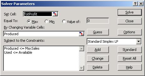
Interpretation 

From the answer report

The optimal solution is to produce 1000 of frame 1, 800 of frame2, and 400 of frame 3; while not to produce any of frame 4. Under this production plan, the maximized profit is $9,200.

We can also see that the labor and metal constraints are binding, which implies that these two constraints are the “Bottlenecks”. They prevent Monet from earning even higher profits.

From the sensitivity report:

The allowable increase/decrease is the range, within witch we can change the constraints, our current optimal solution will still hold.

Reduced Cost is associated with the decision variables. It is defined to be the amount by which the objective function value would be affected if one unit of that decision variable were forced into the optimal solution. In this case, if one more unit of frame 1 is produced, the total profit will drop by $2.

Shadow Price is defined as the change in objective function value resulting from increasing the constraint by 1 unit. However, it is valid only within the allowable increase and decrease range. It reflects the maximum price we would be willing to pay for an additional unit of constraint. In this example, when increase (decrease) 1 unit of labor, the total profit increase (decrease) by $1. In other words, the maximum price to pay for one additional labor is just $1.

Chart

The above chart shows the relationship between labor hours, labor costs, and profit – total profit increases with decreasing labor cost, and that profit increases with labor hours.

Part II  (Example 4.5 and 4.6)

Example 4.5

Situation description and overall objectives

Repco produces three drugs, A, B and C and can sell these drugs in unlimited quantities at different prices. With available labor hours, Repco wants to maximize its sales revenue.

Solution

Traditional Method

The decision variables in the problem are:

The number of units produced for each product, we label them as X_a, X_b, X_c.

The number of units sold of each product, we label them as S_a, S_b, S_c.

The resulting algebraic formulation is shown below:

Maximize 8S_a+70S_b+100S_c         (Revenue Objective)

Subject to: X_a+2X_b+3X_c ≤40   (Labor constraint)

                  -X_a+ 2X_b+S_a ≤0      (Production constraint)

                     -X_b+X_c+S_b≤0       (Production constraint)

S_a-X_a≤0               (Sales Constraints)

S_b-X_b≤0

S_c-X_c≤0

X_a, X_b, X_c³0         (Nonnegativity constraints) 

S_a, S_b, S_c³0     

Spreadsheet Method

See the sheet below

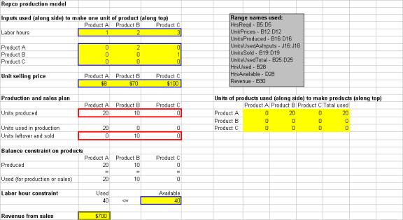
Inputs number of hours need to produce a unit of each product and the number of units of each product needed to manufacture each other product.

Changing Cells the number of units produced and sold and the units used to produce other products

Constraints units used and labor hours are constraints that will be applied in Solver

Target Cell Repco’s revenue from sales

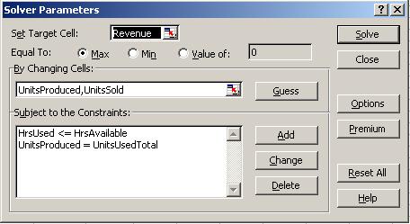
Using Solver

Results Interpretation

The optimal solution for Repco is to produce 20 units of product A and use all of them to produce 10 units of product B. All units of product B are sold. The maximum revenue with current restraints will be $700.

We see all constraints are binding, which implies that we cannot expect more revenue without increasing the resources like labor hours or changing constraints.

Since all the constraints are binding, we cannot see more interesting things from the sensitivity report.

While comparing to the book that used SolverTable, we can achieve the same result by finding that:

All other things unchanged while the price of product C decreased by (-23) which will be effectively increased to 123, we will begin to produce 5.714 units of product C. Thus the total revenue would be $703, slightly better than the original answer.

Example 4.6

Situation description and overall objectives

The toy store, FunToys, projects the monthly cash inflows listed as table below. The store wants to either maximize its cash position at the beginning of January 2001 or minimize the total amount of interest it pays on its loans.

The table of cash flows for FunToys in Year of 2000

	Cash Flow		Cash Flow
January	-12	July	-7
February	-10	August	-2
March	-8	September	15
April	-10	October	12
May	-4	November	-7
June	-5	December	45

Solution

Traditional Algebraic method

In this problem, we need to keep track of the following:

The amount of long-term loan (Lt)

The amount of short-term loan each month (St_i, i=1 ~12)

The monthly interest (MI_i ) and paybacks on the loans (PB_i, i=1~12)

The cash balance at the beginning of each month after the loan (CB_i, i=1~12)

The cash balance at the end of each month (CBE_i, i=1~12)

The algebraic formulation will be as follows:

S_c-X_c≤0

X_a, X_b, X_c³0        

Maximize: CB₁₂

Subject to:  for i=1~12,

       CBE_i ³5000 (End Cash Balance constraints)

 CB_i+1=CBE_i*1.004

 CBE_i+1=CB_i+St_i+1+CF_i+1-MI_i+1-PB_i+1

 MI_i+1=Lt*1%+St_i*1.5%

 PB_i+1=St_i (When i=11, PB₁₂ includes Lt)

As we can see, it is quite difficult to materialize the constraints into traditional algebraic formulas.

Spreadsheet Method

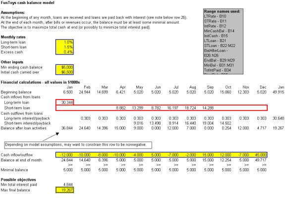
Inputs These include relevant interest rates in the range B9:B11, the minimum cash balance and initial cash in the range B14:B15, and the monthly cash inflows/outflows in the range B28:M28 that were straight from the data table above.

Loan Amounts any trial value in the LTLoan and STLoan range.

Beginning cash balance each month is used to keep track of the cash balance, plus interest, from the previous month.

Loan (and loan interest) paybacks are used to keep track of the loan and loan interest paybacks.

Balance after loan activities is used to calculate the cash balance.

Ending balance is used to calculate the ending balance of each month.

Possible objectives the cell B34 is to calculate the total interest paid and the cell B35 is to calculate the final balance.

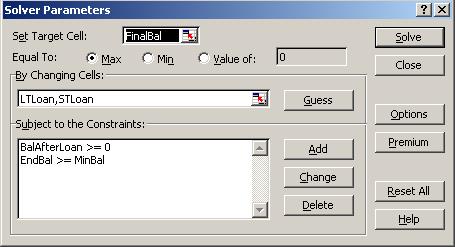
Using Solver

Results Interpretation 

The solution of this problem recommends a long-term loan of $ 30,344 along with short-term loans of various amounts during the 6 months from April to September. At the beginning of January 2001, FunToys’ final cash balance will be $ 19,267, it will have paid back all of its loans, and it has paid $ 4,844 in interest.  

As this financial planning problem is rather complex comparing with the example in Chapter 3, we can expect that the sensitivity report of this problem to be rather confusing since we have more changing variables and constraints. In this situation, it is much better to use SolverTable add-in to get more straightforward analysis.