Guolin Lai

DSC8240 Course Web

Background
Objective Hierarchies
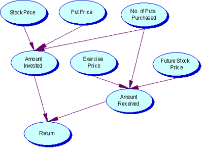
Variables and Attributes
Influence Diagram
Mathematical Representation
Testing and Validation
Implementation and Use

Background
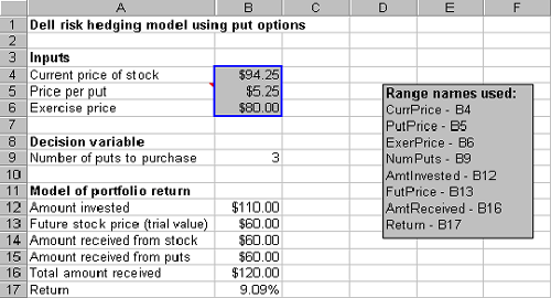
On June 30, 1998 Harry Rockefeller purchases 1 share of Dell Computer for $94.25. However, Harry is worried about the possibility of Dell’s price falling, so he decides to buy some European puts(expiring on November 22, 1998) with an exercise price of $80. Each put is priced at $5.25.

Objective Hierarchies

1. As a function of the number of puts purchases, construct a worst-case and best-case scenario for the return on Harry’s portfolio between June 30, 1998 and November 22, 1998, assuming he sells his stock on the latter date.
2. How does the analysis change if Harry purchases 100 shares rather than 1 share?

Variable and Attributes

Variable	Variable Type	How Measured	Related to
Current Stock Price	Input Variable	$	Amount Invested
Future Stock Price	Decision Variable	$	Amount Received
Price Per Put	Input Variable	$	Amount Invested
Exercise Price	Input Variable	$	Amount Received
Number of Puts to Purchase	Decision Variable	Positive Integer	Amount Invested & Received

Influence Diagram

Mathematical Representation

Amount invested = Current Stock Price + Number of Puts * Price Per Put.
Amount received = Future Stock Price + Number of Puts * IF(Future Stock Price > Exercise Price,0,Exercise Price-Future Stock Price).
Return = (Amount Returned - Amount Invested) / Amount Invested.

Testing and Validation

As a function of the number of puts purchases, construct a worst-case and best-case scenario for the return on Harry’s portfolio between June 30, 1998 and November 22, 1998, assuming he sells his stock on the latter date.

The model shows a positive 9.09% return, but this is obviously a function of the number of puts Harry purchases and the future price of the stock. To examine this dependency more closely, we use a two-way data table to determine the portfolio return for each stock price between $40 and $150 and each number of puts from 0 to 5.

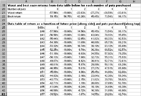
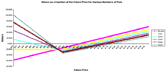
The line chart clearly shows how puts shield Harry from risk if the price of the stock falls precipitously. In fact, the more puts he buys, the more he stands to gain if the price falls significantly. If the price stays about the same or increases, he loses slightly by buying more puts, but the difference is fairly minor. This is illustrated in rows 21 and 22 where we use the MIN and MAX functions to find the worst-case scenario and the best-case returns.

Nevertheless, it is still not clear how many puts Harry should purchase. This depends on the probability distribution of the future stock price. It also depends on Harry’s attitude toward risk.

How does the analysis change if Harry purchases 100 shares rather than 1 share?

If Harry purchases 100 shares of stock rather than 1, we simply multiply the appropriate quantities in the model by 100.
Specifically, his purchase amount for the stock and then amount he receives by selling the stock both increase by a factor of 100. Of course, if he decides to buy, say 3 puts to hedge the risk from owning 1 share of stock, he will probably buy 300 puts if he owns 100 shares.

Implementation and Use

The model can be manipulated in Microsoft Excel.