Guolin Lai
DSC8240 Course Web
Personal Statement
Chapter 1 Summary
Chapter 2 Report
Breakeven Analysis
Price & Demand Relationship
Quantity Discounts Decision
Hedging Investment Risk
Time Value of Money
Enterprise DSS
Time Series Forecasting
DSS Development Project
Simulation Model Examples
Government Contract Bidding
GFAuto Model
Customer Loyalty
Game of Craps
Monte Carlo Simulation
Optimization Modeling
Term Project
Business Intelligence Research
Background
Objective Hierarchies
Variables and Attributes
Influence Diagram
Mathematical Representation
Testing and Validation
Implementation and Use
Background
Acron is a large drug company. One of its new drugs, Niagara, is coming
to market and Acron needs to determine how much annual production capacity
to build for this drug. Government regulations make it difficult to add
capacity at a later date, so Acron must determine a capacity recommendation
before the drug comes to market. The drug will be sold for 20 years before
it comes off patent. After the 20 years, the rights to produce the drug
are virtually worthless.
Acron has made the following assumptions:
- Year 1 demand will be 10,000 units.
- During years 2-6, annual growth of demand will be 15%.
- During years 7-20, annual growth of demand will be 5%.
- It costs $6, payable at the end of year 1, to build each unit of annual production capacity. The cost of the building capacity is deprecisted on a straight-line 5-year basis.
- During year 1, Niagara will sell for $8 per unit and will incur a variable cost $5 to produce.
- The cost of maintaining a unit capacity during year 1 is $1.
- The sales price, unit variable cost, and unit capacity maintenance cost will increase by 5% per year.
- Profits are taxed at 40%.
- All cash flows are assumed to occur at the end of each year, and the
corporate discount rate is 10%.
Objective
Hierarchies
Acron wants to develop a spreadsheet model of its 20-year cash flows.
Then it wants to answer the following questions.
- What capacity level should be chosen?
- How does a change in the discount rate affect the optimal capacity level?
- How realistic is the model?
|
Variable
|
Variable Type
|
How Measured
|
Related to
|
| Year 1 Demand | Input Variable | Numerical Value | Year 2 - 20 Demand |
| Year 2 - 6 Growth Rate | Input Variable | % | Year 2 - 6 Demand |
| Year 7 - 20 Growth Rate | Input Variable | % | Year 7 - 20 Demand |
| Unit Cost of Production Capacity | Input Variable | $ | Building Cost |
| Depreciation Rate | Input Variable | % | Depreciation |
| Unit Price | Input Variable | $ | Revenue |
| Unit Variable Cost | Input Variable | $ | Variable Cost |
| Unit Capacity Maintenance Cost | Input Variable | $ | Maintenance Cost |
| Inflation Rate | Input Variable | % | Unit Price, Unit Variable Cost, Unit Capacity Maintenance Cost (Year 2 - 20) |
| Tax Rate | Input Variable | % | After Tax Profit |
| Discount Rate | Input Variable | % | Net Present Value |
| Capacity Level | Decision Variable | Numerical Value | Units Sold |
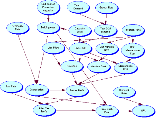
Building cost = Unit Cost of Productino Capacity * Capacity Level
Depreciation = Depreciation Rate * Building Cost
Demand 2 - 6 = 1st year demand * (1 + year 2-6 growth rate)
Demand 7 - 20 = 6th year demand * (1 + year 7-20 growth rate)
Units Sold = Min(Capacity Level, Demand)
Unit Price = Unit Price * ( 1 + inflation rate)
Unit Variable Cost = Unit Variable Cost * (1 + inflation rate)
Unit Maintenance Cost = Unit Maintenance Cost * (1 + inflation rate)
Revenue = Units Sold * Unit Price
Variable Cost = Units Sold * Unit Variable Cost
Maintenance Cost = Units Sold * Unit Maintenance Cost
Pretax Profit = Revenue - Depreciation - Variable Cost - Maintenance Cost
After Tax Profit = IF(Pretax Profit < 0, Pretax Profit, Pretax Profit
*(1-Tax Rate))
Free Cash Flow(1st year)= Depreciation + After Tax Profit - Building Cost
Free Cash Flow(2nd - 5 th year)= Depreciation + After Tax Profit
Free Cash Flow(6th - 20th year)= After Tax Profit
NPV(Discount Rate,Free Cash Flow)
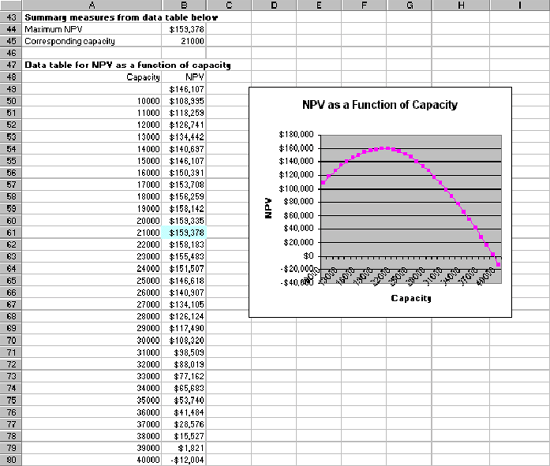
What capacity level should be chosen?
It is useful to create the data table and corresponding chart. These show how NPV varies for different levels of capacity. More specifically, it indicates that Acron can maximize its NPV by using a capacity level of 21,000 units.
How does a change in the discount rate affect the optimal capacity level?
To answer the questions, we build the two-way data table and corresponding chart.
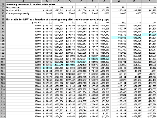
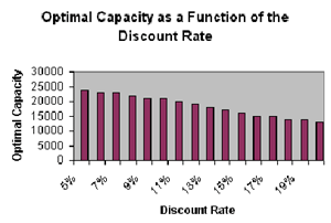
As we see, larger discount rates typically result in lower NPVs because
future cash flows are discounted more heavily.
Beyond this, the chart shows how the optimal decreases as the discount
rate increases.The reasoning is basically that “bad” things,
especially building costs, tend to occur early, whereas “good”
things tend to occur later on. A higher discount rate magnifies the bad
things relative to the good things, so it induces the company to build
less capacity.
How realistic is the model?
Probably the major flaw is that we have ignored uncertainty. It is clear
that demand, future prices and future costs are highly uncertain. Of course,
there are almost always ways to make any model more realistic – at
the cost of increased complexity.
For example, we could model the impact of competition on Niagara’s
profitability. We could also realize that Acron’s pricing policy
is not set in stone and the price it charges will influence the likelihood
that competition will enter the market.
Finally, Acron could probably add capacity in the future if it is experiencing
larger than expected demand. However, it is important to realize that
future flexibility in decision making has an impact on the correct decision
for today.
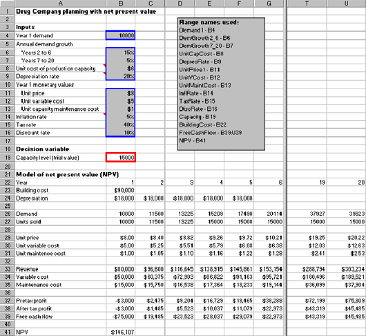
The model can be manipulated in Microsoft Excel.